
A debugging guide for image segmentation models
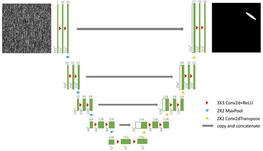
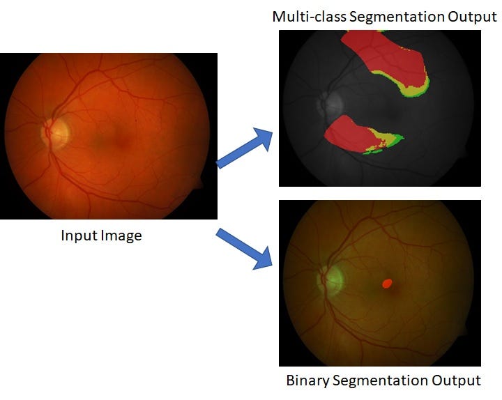
U-net Model from Binary to Multi-class Segmentation Tasks (Image by Author)
Image semantic segmentation is one of the most significant areas of research and engineering in the computer vision domain. From segmenting pedestrians and cars for autonomous drive [1] to segmentation and localization of pathology in medical images [2], there are several use-cases of image segmentation. With the wide-spread use of deep learning models for end-to-end delivery for machine learning (ML) models, the U-net model has emerged as a scalable solution across autonomous drive and medical imaging use-cases [3–4]. However, most existing papers and methods implement binary classification tasks for detecting objects/regions of interest over the backgrounds [4]. In this hands-on tutorial we will review how to start from a binary semantic segmentation task and transfer the learning to suit multi-class image segmentation tasks.
One of the biggest frustrations for an ML engineer in their daily workflow is to spend hours training a ML model, only to end up with results that make no sense, such as outputs of Not-a-Number (NaN) or images with all 0 values. In this tutorial, we will learn the step-by-step process to begin the process of ML model building from existing works (papers/codebases) and to modify it significantly to suit your own data needs through an example where a binary U-net model is extended to multi-class semantic segmentation.
The U-net model represents encoder and decoder layers in combination with skip connections between the encoded and the respective decoded layers, as shown in Fig. 1. The primary advantage of the skip connections is that it combines the encoded and decoded outcomes per depth layer to enable consistent separation between the foreground (pixels that need to be output as white) vs. the background (pixels that need to be output as dark).
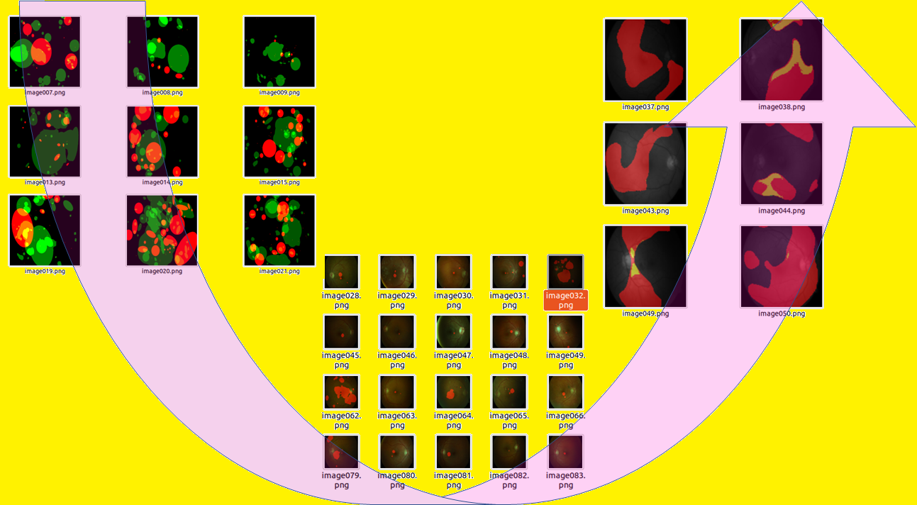
With the ultimate goal to optimally tune the model hyper-parameters for a new codebase, we begin with the existing U-net code base in [5] that uses binary semantic segmentation on retinal image data set [6] to modify the codebase for multi-class classification of retinal image pathology using the DIARETDB1 data set [7–8]. The pathology categories are bright lesions (BL) indicated by “hardexudates” and “softexudates” and red lesions indicated by “hemorrhages” and “redsmalldots” [8].
The three major steps in the data model transformation are as follows: 1) Data Preparation 2) Data Model and Process 3) Outcomes and Metrics.
Step 1: Data Preparation: From Binary to Multi class
The first step in building an end-to-end ML model is benchmarking, which involves replicating an existing codebase/paper as much as possible. If this necessitates modification of the current data set to resemble the existing work’s data, then that should be done.
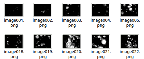
Starting with the U-net code base in [5], for the multi-class pathology classification task we have at hand, we first replicate the U-net codebase [5] for a single pathology, hemorrhage detection task.
The resulting hemorrhage labels are shown in Fig. 2 below.
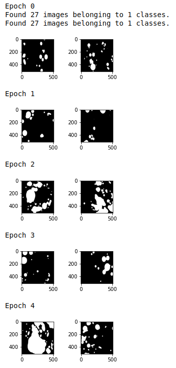
Medical image datasets often pose the problem of “small data challenge”, where there are limited samples to train on. To remedy this problem, image data augmentation using Keras is frequently used. The goal with this approach is to generate multiple zoomed in/out, rotated, panned in/out equivalents of a single image and its mask at run time.
One important consideration when training on data sets with few samples is that a trained model has a tendency to get heavily biased by class imbalance in sample pixels. For example, the data set in [8] contains 89 images, but only about 30 images contain large regions of interest corresponding to pathology. The remaining labelled images are mostly Y=0. Therefore, if a model is trained with all images, there will be a tendency to predict most images as Y=0, which means the pathology will mostly get missed. To avoid this issue, and to separate the image data into train and test sets, we use image ID 1–27 for training, while images 28–89 are used for testing only.
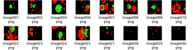
When migrating to multi-class segmentation from binary segmentation, the first requirement is to format the data appropriately. Given original image X and labels Y, the dimensions for X are [m x m x r] and Y are [m x m x d], where the image dimensions input to the U-net model are m=256, r=3 (RGB image) and d represents the number of classes for the multi-class classification (d=4, here). The requirement for a U-net model is that the input and output must belong to the same domain/dimensions, which is [m x m] in this case. The only difference is that the input X can be a color or grayscale image, while the output Y represents binary image planes corresponding to each pathology mask. So each output image plane represents a one vs all classification at a pixel level.
The outcome is shown in Fig 3 below.
Step 2: Data Model and Process
The key tasks for training an optimal ML model involve hyper-parameter optimization, which involves selecting the best set of parameters that ensure well fit weights and biases for the deep learning U-net model. We perform hyper-parameter selection for the following:
- Compiler (Adam)
- Learning rate (0.0001)
- Accuracy metric: Dice coefficient [9] to be maximized
- Loss metric: negative Dice coefficient (to be minimized)
Other options for the accuracy metric and loss metric are ‘accuracy’ and ‘categorical_crossentropy’ with ‘sample_weights=temporal’ [10] to cater to data imbalance.
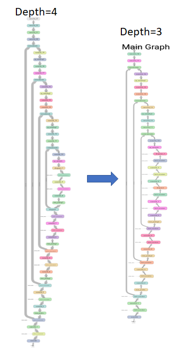
Another model parameter that needs to be tuned is the model complexity (i.e. the training complexity imposed by size of the U-net). Thus, there is a need to train on deep U-nets (depth=4) and shallow U-nets (depth=3) with graphs as shown below. The model with fewer parameters is typically optimal for the “small data challenges”. The variations in the models with depth 3 and 4 can be seen in [11].
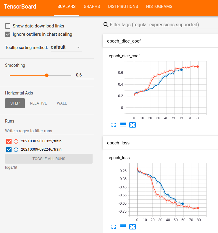
At the end of model training, the loss curves demonstrate how effective the training process was. The loss curves for our implementation are shown in Fig 5 below.
Step 3: Outcomes and Metrics
Once the model is trained, the final task is to evaluate on test data. Qualitatively, the outcomes are shown in Fig. 6.
For quantitative assessment, we consider the following metrics: Precision, Recall, Accuracy, Intersection over Union (IoU) and F1 score [9] [12] as shown below after the binary segmentation.

The outputs can be found in the Github [11].
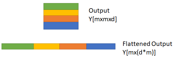
Since the output Y has ‘d’ planes, the first task is to flatten the planes as shown in [13] and Fig 7., followed by computing the combined Dice coefficient. Thus, the Dice coefficient of multi-class segmentation is additive over all the output planes and hence it can exceed the value 1.
Finally, the quantitative evaluation of the multi-class segmentation involves macro and micro-level metrics being reported. While macro level precision, recall, accuracy, IOU and F1 score weights all the classes equally, micro level metrics are preferable in situations with class imbalance to provide a weighted outcome as seen in [14].
Conclusions
Transfer learning from existing ML models to new data sets and use-cases requires a strategic workflow to ensure optimal data modeling. The key is in structuring the workflow as: Data, Processes and Outcomes. Using the step-by-step guide presented in this tutorial, it will be possible to extend the U-net model to not only other binary but multi-class classification tasks. Other codebases that deal with multi-class segmentation are in [15].
To further improve the performances shown in this tutorial, larger image sizes, and one vs all segmentation approaches can be combined for all the red and bright lesions. Also, to extend the tutorial to more classes, the augmented outcomes ‘Y’ can be saved as .npy files rather than images and the load command can be used to load the augmented data rather than the load_img (that inputs 3D image data only.) Using the proposed methods, readers should now be equipped with the means and methods to learn from existing code bases and modify them to their own needs while extending the scope of the models and methods.
References
[1] Piccoli, Francesco, et al. “FuSSI-Net: Fusion of Spatio-temporal Skeletons for Intention Prediction Network.” arXiv preprint arXiv:2005.07796 (2020).
[2] Roychowdhury, Sohini. “Few Shot Learning Framework to Reduce Inter-observer Variability in Medical Images.” arXiv preprint arXiv:2008.02952 (2020).
[3]Zhang, Zhengxin, Qingjie Liu, and Yunhong Wang. “Road extraction by deep residual u-net.” IEEE Geoscience and Remote Sensing Letters 15.5 (2018): 749–753.
[4]M. Larkin. “Check out our graduates’ final projects”.[Online] https://blog.fourthbrain.ai/check-out-our-graduates-final-projects?utm_campaign=Project%20Presentation%20Day&utm_source=tds-blog&utm_medium=blog&utm_term=mldebugging-guide&utm_content=ml-debugging-guide
[5] S. Roychowdhury. “Unet for Medical Image Segmentation using TF 2.x” [Online]https://github.com/sohiniroych/Unet-using-TF2
[6]A. Hoover. “The STARE Project”. [Online] https://cecas.clemson.edu/~ahoover/stare/probing/index.html
[7] Roychowdhury, Sohini, Dara D. Koozekanani, and Keshab K. Parhi. “DREAM: diabetic retinopathy analysis using machine learning.” IEEE journal of biomedical and health informatics 18.5 (2013): 1717–1728.
[8]Singh, Ramandeep, et al. “Diabetic retinopathy: an update.” Indian journal of ophthalmology 56.3 (2008): 179.
[9]E Tiu. “Metrics to Evaluate your Semantic Segmentation Model”. [Online] https://towardsdatascience.com/metrics-to-evaluate-your-semantic-segmentation-model.
[10] Stack Overflow [Online]U-net: how to improve accuracy of multiclass segmentation?
[11] S. Roychowdhury. “U-net for multiclass semantic segmentation”. [Online] https://github.com/sohiniroych/U-net-for-Multi-class-semantic-segmentation
[12] H. Kumar. Evaluation metrics for object detection and segmentation: mAP [Online] https://kharshit.github.io/blog/2019/09/20/evaluation-metrics-for-object-detection-and-segmentation
[13] https://stackoverflow.com/questions/43237124/what-is-the-role-of-flatten-in-keras
[14] Data Science Stack Exchange. Micro Average vs Macro average Performance in a Multiclass classification setting [Online]: https://datascience.stackexchange.com/questions/15989/micro-average-vs-macro-average-performance-in-a-multiclass-classification-settin
[15]H Tony. Unet : multiple classification using Keras [online] https://github.com/HZCTony/U-net-with-multiple-classification
Originally published at: https://towardsdatascience.com/a-machine-learning-engineers-tutorial-to-transfer-learning-for-multi-class-image-segmentation-b34818caec6b